
A review on the stochastic simulation of rainfall process data for soil erosion assessment
Received date: 2019-09-22
Request revised date: 2020-05-02
Online published: 2020-12-28
Supported by
National Natural Science Foundation of China(41301281)
Copyright
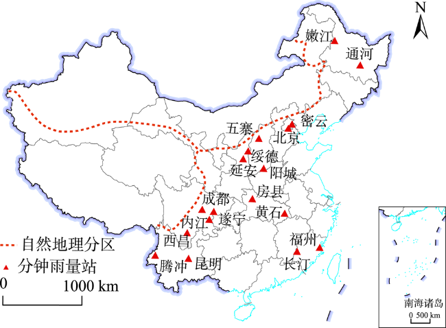
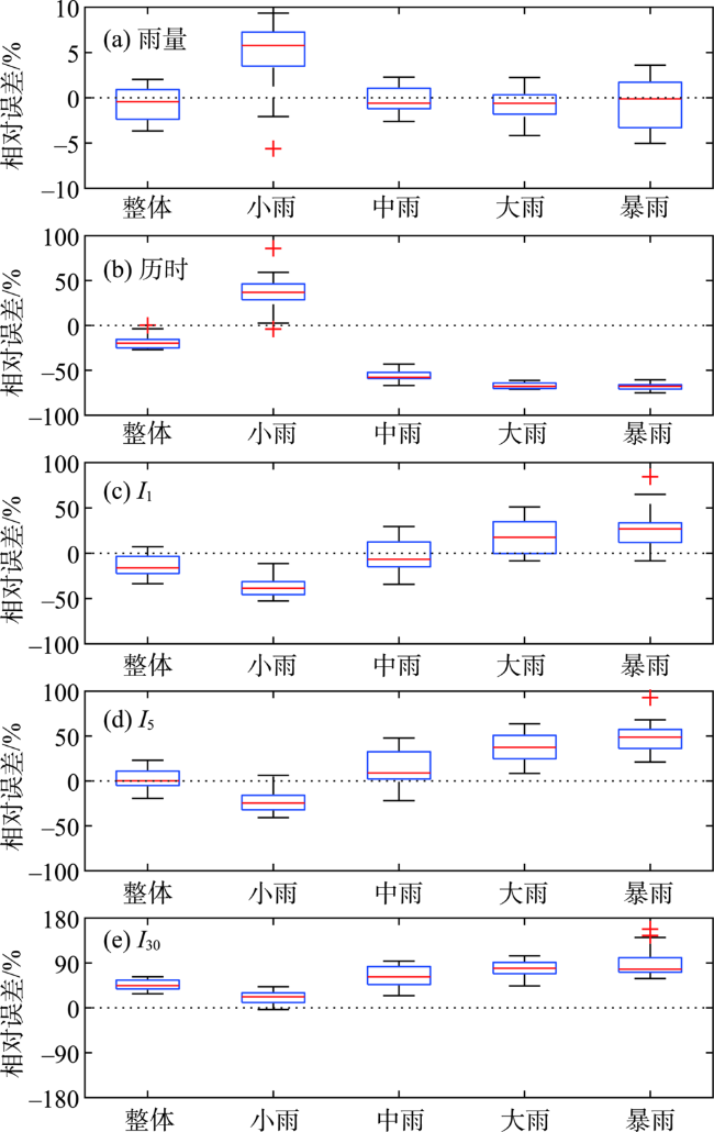
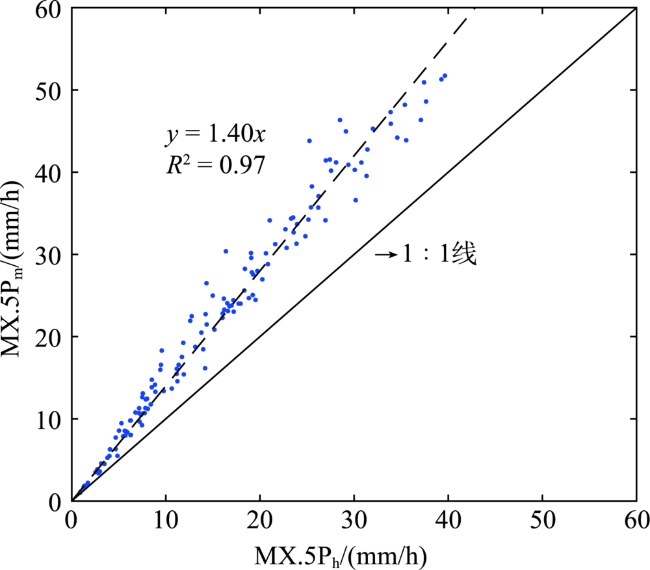
Soil erosion is one of the most serious environmental problems in China. Soil erosion model is an efficient tool for diagnosing and preventing soil erosion. Stochastic simulation of precipitation can generate synthetic input data for soil erosion models when observation data are absent. This study summarized the main progress of rainfall process stochastic simulation in existing studies. One-minute resolution rainfall data were collected from 18 weather stations distributed in the main water erosion areas to analyze the characteristics of the storm process and calibrate, evaluate, and develop CLImate GENerator (CLIGEN) stochastic models for China. The main results are as follows: 1) Minimum inter-event time (MIT) for separating precipitation events from continuous precipitation recording ranged from 7.6 h to 16.6 h, with an average of 10.7 h. The MIT values calculated from 1-minute data and hourly data were not significantly different. Storm process characteristics such as the amount, duration, average intensity, and peak intensity of precipitation were sensitive to the variation of MIT values when the MIT values were smaller than 6 h, which suggests that the comparison of storm process characteristics for different storms and areas should use the same MIT value. 2) Events with peak intensity occurring in the first half of the duration of an event were dominant, which accounted for more than 65% of the total events and they were characterized by relatively short duration and greater intensity, comparing with events whose peak intensity fell in the second half of the duration of the events. 3) Weather generator CLIGEN in the Water Erosion Prediction Project (WEPP) soil erosion model can satisfactorily simulate the daily precipitation amounts (P), but it underestimated the storm duration (D) and overestimated the maximum 30-minute intensity (I30). The direction and degree of the bias for D and I30 were not consistent for different groups classified by different precipitation amounts. 4) A method was developed to use hourly precipitation data to prepare the TimePk and MX.5P parameters for CLIGEN input files for the generation of storm process data in the absence of high resolution hyetography precipitation data. More efforts are needed to improve the simulation of precipitation extremes and develop multi-site and multi-variable stochastic models conditioned on weather types in the future.
YIN Shuiqing , WANG Wenting . A review on the stochastic simulation of rainfall process data for soil erosion assessment[J]. PROGRESS IN GEOGRAPHY, 2020 , 39(10) : 1747 -1757 . DOI: 10.18306/dlkxjz.2020.10.013
表1 常见次降雨过程特征参数Tab.1 Characteristic parameters of the storm event process |
| 指标 | 常用符号 | 单位 | 定义 |
|---|---|---|---|
| 最小降雨间歇 | MIT | h | 分割次降雨的最小时间间隔,当干期小于该临界值,则合并为1次降雨;否则划分为2次独立的次降雨事件 |
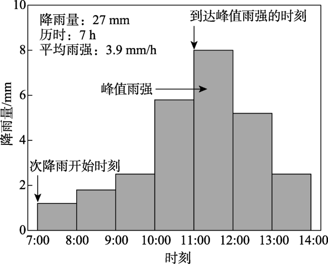
| 次降雨量 | P | mm | 一次降雨过程内产生的降雨量总和 |
| 次降雨历时 | D | h | 次降雨过程的总时长,次降雨过程内部的干期成为次降雨历时的一部分 |
| 次降雨平均雨强 | I | mm/h | 次降雨量除以次降雨历时 |
| 次降雨峰值雨强 | I1、I5、I30 | mm/h | 次降雨过程中最大的时段雨强,比如最大1 min、5 min、30 min雨强,最大小时雨强等 |
| 到达峰值雨强的时刻 | tp | h | 从降雨开始至到达峰值雨强时刻的时间 |
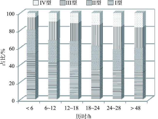
| 时程雨型 | 降雨过程中雨量随历时的分配,反映了降雨发生、发展和消亡的过程 |
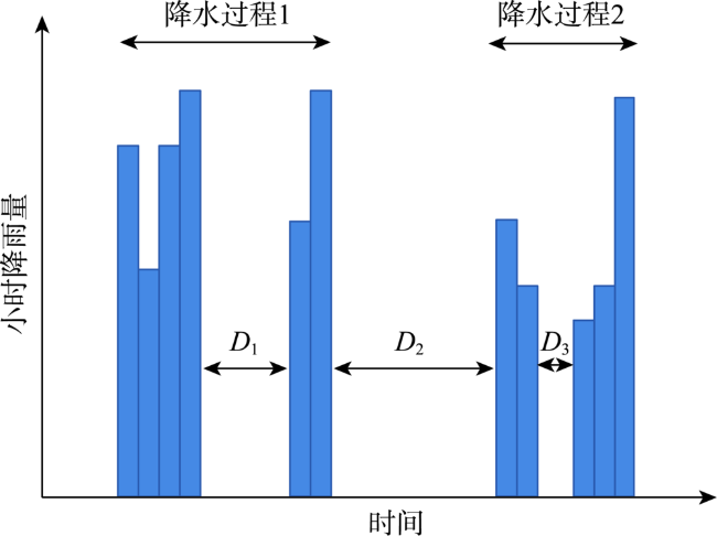
图1 最小降雨间歇示意图注:D1、D2和D3为干期(降雨间歇),D1和D3小于最小降雨间歇;D2大于等于最小降雨间歇。 Fig.1 Illustration of the MIT |
表2 基于分钟与小时资料通过指数方法计算得到的18站MITexpTab.2 MIT of 18 stations calculated using the exponential method based on 1-minute and hourly precipitation data respectively |
| 站名 | 基于分钟资料计算 | 基于小时资料计算 | 相对偏差/% |
|---|---|---|---|
| 嫩江 | 10.2 | 9.2 | -9.8 |
| 通河 | 12.9 | 11.9 | -7.8 |
| 五寨 | 7.9 | 6.8 | -13.9 |
| 绥德 | 8.9 | 8.0 | -10.1 |
| 延安 | 9.0 | 7.8 | -13.3 |
| 阳城 | 8.6 | 7.7 | -10.5 |
| 密云 | 10.1 | 9.3 | -7.9 |
| 北京 | 11.9 | 11.9 | 0 |
| 成都 | 7.9 | 7.1 | -10.1 |
| 西昌 | 9.1 | 8.4 | -7.7 |
| 腾冲 | 11.1 | 10.8 | -2.7 |
| 昆明 | 12.7 | 11.8 | -7.1 |
| 房县 | 7.8 | 6.8 | -12.8 |
| 遂宁 | 8.2 | 7.6 | -7.3 |
| 内江 | 7.6 | 6.9 | -9.2 |
| 黄石 | 14.7 | 14.0 | -4.8 |
| 福州 | 16.6 | 15.6 | -6.0 |
| 长汀 | 16.5 | 15.6 | -5.5 |
| 平均值 | 10.7 | 9.8 | -8.1 |
| 标准差 | 2.9 | 3.0 | 3.6 |
注:为便于各站比较,表中各指标基于所有站点共有的5—9月资料进行计算。 |
表3 最小降雨间歇分别为1 h、2 h、6 h 和各站MITexp时,次降雨过程特征参数的平均值统计特征Tab.3 Mean storm properties when using 2 h, 6 h, 10 h, and exponential method-derived MIT values to delineate independent storms |
| 站点 | 雨量P/mm | 历时D/h | 平均雨强I/(mm/h) | 峰值雨强I30/(mm/h) | |||||||||||||||
|---|---|---|---|---|---|---|---|---|---|---|---|---|---|---|---|---|---|---|---|
| 2 h | 6 h | 10 h | MITexp | 2 h | 6 h | 10 h | MITexp | 2 h | 6 h | 10 h | MITexp | 2 h | 6 h | 10 h | MITexp | ||||
| 嫩江 | 6.3 | 9.1 | 11.3 | 11.3 | 6.6 | 15.8 | 24.1 | 24.5 | 1.3 | 0.8 | 0.7 | 0.7 | 5.5 | 6.7 | 7.6 | 7.6 | |||
| 通河 | 6.3 | 8.8 | 10.8 | 12.0 | 5.5 | 11.7 | 18.1 | 22.5 | 1.6 | 1.1 | 0.8 | 0.7 | 5.7 | 6.7 | 7.5 | 7.8 | |||
| 五寨 | 6.3 | 8.1 | 9.1 | 8.6 | 5.2 | 8.3 | 10.8 | 9.5 | 1.7 | 1.5 | 1.4 | 1.5 | 4.9 | 5.7 | 6.0 | 5.8 | |||
| 绥德 | 7.1 | 9.1 | 10.1 | 9.8 | 5.6 | 9.2 | 11.6 | 10.8 | 1.9 | 1.8 | 1.7 | 1.7 | 5.4 | 6.3 | 6.7 | 6.6 | |||
| 延安 | 8.2 | 10.3 | 11.4 | 11.1 | 6.7 | 10.2 | 12.9 | 12.2 | 1.9 | 1.7 | 1.5 | 1.6 | 5.7 | 6.5 | 6.9 | 6.8 | |||
| 阳城 | 9.5 | 12.0 | 13.3 | 13.0 | 8.4 | 13.0 | 15.9 | 15.2 | 1.4 | 1.3 | 1.2 | 1.2 | 6.5 | 7.6 | 8.1 | 8.0 | |||
| 密云 | 10.5 | 12.8 | 14.3 | 14.4 | 5.2 | 7.9 | 10.2 | 10.2 | 2.8 | 2.6 | 2.5 | 2.4 | 9.2 | 10.5 | 11.2 | 11.3 | |||
| 北京 | 9.6 | 12.3 | 13.6 | 14.5 | 4.7 | 8.3 | 10.7 | 12.6 | 2.4 | 2.1 | 2.0 | 1.8 | 8.2 | 9.7 | 10.4 | 10.7 | |||
| 成都 | 10.1 | 12.7 | 14.7 | 13.6 | 7.6 | 12.3 | 16.3 | 14.2 | 1.6 | 1.3 | 1.2 | 1.2 | 7.4 | 8.5 | 9.3 | 8.9 | |||
| 西昌 | 8.4 | 12.0 | 14.4 | 14.3 | 5.8 | 10.8 | 14.9 | 14.7 | 1.5 | 1.4 | 1.3 | 1.3 | 5.7 | 7.4 | 8.2 | 8.2 | |||
| 腾冲 | 5.6 | 9.3 | 13.4 | 14.8 | 3.4 | 8.3 | 15.5 | 18.2 | 1.9 | 1.6 | 1.5 | 1.4 | 5.1 | 6.7 | 7.9 | 8.3 | |||
| 昆明 | 6.9 | 11.5 | 15.1 | 17.1 | 5.3 | 13.6 | 21.3 | 26.2 | 1.7 | 1.3 | 1.1 | 1.1 | 6.3 | 8.4 | 9.8 | 10.4 | |||
| 房县 | 9.2 | 12.0 | 13.8 | 13.0 | 7.9 | 12.3 | 15.9 | 14.3 | 1.5 | 1.4 | 1.4 | 1.4 | 6.1 | 7.3 | 8.1 | 7.8 | |||
| 遂宁 | 10.2 | 12.3 | 13.7 | 13.1 | 7.3 | 9.8 | 12.1 | 11.0 | 1.8 | 1.7 | 1.6 | 1.7 | 7.2 | 8.2 | 8.8 | 8.5 | |||
| 内江 | 10.6 | 13.8 | 15.5 | 14.8 | 6.7 | 10.5 | 13.2 | 12.1 | 1.9 | 1.8 | 1.7 | 1.7 | 7.5 | 8.9 | 9.6 | 9.3 | |||
| 黄石 | 14.0 | 18.4 | 21.0 | 23.2 | 6.9 | 10.7 | 13.5 | 16.4 | 2.6 | 2.6 | 2.4 | 2.4 | 9.8 | 11.7 | 12.6 | 13.4 | |||
| 福州 | 12.4 | 18.2 | 22.8 | 28.4 | 10.1 | 19.9 | 28.4 | 39.9 | 1.4 | 1.0 | 1.0 | 0.9 | 8.5 | 10.7 | 12.4 | 13.9 | |||
| 长汀 | 12.9 | 17.9 | 21.3 | 26.8 | 8.5 | 15.4 | 21.0 | 30.0 | 1.9 | 1.6 | 1.5 | 1.5 | 10.2 | 12.0 | 13.1 | 14.6 | |||
| 平均值 | 9.1 | 12.3 | 14.4 | 15.2 | 6.5 | 11.6 | 15.9 | 17.5 | 1.8 | 1.6 | 1.5 | 1.5 | 6.9 | 8.3 | 9.1 | 9.3 | |||
表4 基于不同的最小降雨间歇划分次降雨过程得到的次降雨特征参数18站均值的配对t检验结果Tab.4 Probability value of two-sample tests conducted for storm properties derived from commonly used MIT values |
| 降雨特征指标 | 2 h与6 h | 2 h与10 h | 2 h与MITexp | 6 h与10h | 6 h与MITexp | 10 h与MITexp |
|---|---|---|---|---|---|---|
| 雨量P | 0.002 | <0.001 | <0.001 | 0.072** | 0.057** | 0.626** |
| 历时D | <0.001 | <0.001 | <0.001 | 0.004 | 0.007 | 0.508** |
| 平均雨强I | 0.134** | 0.033* | 0.026* | 0.528** | 0.467** | 0.922** |
| 峰值雨强I30 | 0.027* | 0.001 | 0.002 | 0.235** | 0.190** | 0.805** |
注:*、**分别表明2列样本在0.01、0.05的显著水平下差异不显著。 |
感谢国家自然科学基金委员会地学部冷疏影研究员、北京大学遥感与地理信息系统研究所范闻捷副教授在本文写作过程中给予的支持和帮助,感谢匿名审稿人专业且富有建设性的修改建议。本文在撰写过程中得到了北京师范大学谢云教授的帮助,在此一并表示衷心的感谢!
| [1] |
刘宝元, 谢云, 张科利. 土壤侵蚀预报模型 [M]. 北京: 中国科学技术出版社, 2001.
[
|
| [2] |
|
| [3] |
陈杰, 许崇育, 郭生练, 等. 统计降尺度方法的研究进展与挑战[J]. 水资源研究, 2016,5(4):299-313.
[
|
| [4] |
刘昌明, 刘文彬, 傅国斌, 等. 气候影响评价中统计降尺度若干问题的探讨[J]. 水科学进展, 2012,23(3):427-437.
[
|
| [5] |
范丽军, 符淙斌, 陈德亮. 统计降尺度法对未来区域气候变化情景预估的研究进展[J]. 地球科学进展, 2005,20(3):320-329.
[
|
| [6] |
|
| [7] |
|
| [8] |
殷水清, 谢云, 陈德亮, 等. 日以下尺度降雨随机模拟研究进展[J]. 地球科学进展, 2009,24(9):981-989.
[
|
| [9] |
|
| [10] |
|
| [11] |
|
| [12] |
|
| [13] |
|
| [14] |
|
| [15] |
|
| [16] |
|
| [17] |
|
| [18] |
|
| [19] |
|
| [20] |
|
| [21] |
|
| [22] |
|
| [23] |
|
| [24] |
|
| [25] |
|
| [26] |
USDA-Agricultural Research Service. Science documentation Revised Universal Soil Loss Equation Version 2 [M/OL]. . Washington D C, USA:USDA-ARS, 2013.
|
| [27] |
|
| [28] |
|
| [29] |
殷水清, 王杨, 谢云, 等. 中国降雨过程时程分型特征[J]. 水科学进展, 2014,25(5):617-624.
[
|
| [30] |
|
| [31] |
|
| [32] |
|
| [33] |
|
| [34] |
|
| [35] |
|
| [36] |
|
| [37] |
|
| [38] |
|
| [39] |
|
| [40] |
|
| [41] |
|
| [42] |
|
| [43] |
|
| [44] |
赵松乔. 中国综合自然地理区划的一个新方案[J]. 地理学报, 1983,38(1):1-10.
[
|
| [45] |
|
| [46] |
|
| [47] |
|
| [48] |
|
| [49] |
|
| [50] |
|
| [51] |
|
| [52] |
|
| [53] |
|
| [54] |
|
| [55] |
|
| [56] |
|
| [57] |
|
| [58] |
|
| [59] |
|
/
| 〈 |
|
〉 |