
Interpolation methods comparison of VIIRS/DNB nighttime light monthly composites: A case study of Beijing
Received date: 2018-04-03
Request revised date: 2018-09-16
Online published: 2019-01-22
Supported by
Strategic Priority Research Program of Chinese Academy of Sciences, No. XDA20010203
Key Project of the Chinese Academy of Sciences, No. ZDRW-ZS-2017-4
Fundamental Research Funds for the Central Universities, No. 2018CXZZ003.
Copyright
Comparing with nighttime light data acquired by the Defense Meteorological Satellite Program's Operational Linescan System (DMSP/OLS), nighttime light data sensed by the Visible Infrared Imaging Radiometer Suite Day/Night Band (VIIRS/DNB) have a higher spatial resolution and finer temporal resolution. VIIRS/DNB nighttime light data also have a substantial number of improvements in terms of accuracy and in-flight calibrations. As a result, VIIRS/DNB nighttime light data become a new research hotspot rapidly. Even so, VIIRS/DNB nighttime light data are vulnerable to stray light and contain a large number of distorted values in mid and high latitudes, especially in summer. Therefore, this study took Beijing as an example and adopted cubic spline interpolation (spline), cubic Hermite interpolation (Hermite), gray model (GM), and triple exponential smoothing (exponent) to interpolate default data of May to July 2015, and then compared the results of these four interpolation algorithms. The result shows that: 1) With regard to abnormal values, Hermite does not produce any abnormal value, while the other three algorithms generate few such values (0.02%~1.34%). 2) Comparing with the reference data—the Visible Infrared Imaging Radiometer Suite Cloud Mask Stray Light (VCMSL) version, the interpolation result of Hermite is closest to the reference, and the GM result is least close to the reference. 3) In terms of computing time, all of these four algorithms are easy to be programmed and calculated, but the exponential smoothing method has to calculate smoothing parameter repeatedly and therefore it will spend much more time than the other three algorithms. In conclusion, a comprehensive assessment shows that when the two time periods before and after the interpolation months both have enough original data, Hermite will be the best choice because of its great interpolation performance, no overshoots, and fast calculation speed. Spline takes the second place. When only one side of the interpolation months has adequate data, GM and exponent methods both can be used. The GM calculation runs fast but the interpolation result is not optimal, and exponent calculation runs slow but the algorithm interpolates well.
CHEN Mulin , CAI Hongyan . Interpolation methods comparison of VIIRS/DNB nighttime light monthly composites: A case study of Beijing[J]. PROGRESS IN GEOGRAPHY, 2019 , 38(1) : 126 -138 . DOI: 10.18306/dlkxjz.2019.01.011
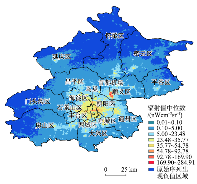
Fig.1 Visible Infrared Imaging Radiometer Suite Cloud Mask (vcm) composites’ median value of August 2014 to April 2016 (excluding May to July 2015)图1 2014年8月至2016年4月(不包含2015年5—7月)“vcm”产品辐射值中位数图 |
Tab.1 Distribution of interpolation anomaly (nWcm-2sr-1)表1 插补结果异常值分布 |
| 插补方法 | 5月 | 6月 | 7月 | |||||
|---|---|---|---|---|---|---|---|---|
| <0 均值 (个数) | >285 均值 (个数) | <0 均值(个数) | >285 均值(个数) | <0 均值(个数) | >285 均值(个数) | |||
| 三次样条插值 | -0.15 (899) | 312.11 (6) | -0.20 (1341) | 315.51 (3) | -0.21 (819) | 301.88 (2) | ||
| 三次Hermite插值 | 0 (0) | 0 (0) | 0 (0) | 0 (0) | 0 (0) | 0 (0) | ||
| 灰色预测模型 | -9.04 (16) | 0 (0) | -10.88 (16) | 0 (0) | -14.71 (14) | 0 (0) | ||
| 三次指数平滑 | -0.08 (710) | 297.36 (2) | -0.11 (850) | 290.64 (2) | -0.10 (1447) | 297.76 (4) | ||
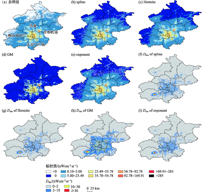
Fig.2 Interpolation results of May: (a) is Visible Infrared Imaging Radiometer Suite Cloud Mask Stray Light (vcmsl) of May; (b) and (f) are cubic spline interpolation (spline) method's interpolation result and distribution of Dabs, respectively; (c) and (g) are cubic Hermite interpolation (Hermite) method's interpolation result and distribution of Dabs, respectively; (d) and (h) are gray model's (GM) interpolation result and distribution of Dabs, respectively; (e) and (i) are triple exponential smoothing (exponent) method's interpolation result and distribution of Dabs, respectively图2 5月份插补结果对比图:(a)为5月份“vcmsl”参照值;(b)与(f)分别为三次样条插值(spline)方法的插补结果及其Dabs分级;(c)与(g)分别为三次Hermite插值(Hermite)的插补结果及其Dabs分级;(d)与(h)分别为灰色预测模型(GM)的插补结果及其Dabs分级;(e)与(i)分别为三次指数平滑(exponent)方法的插补结果及其Dabs分级 |
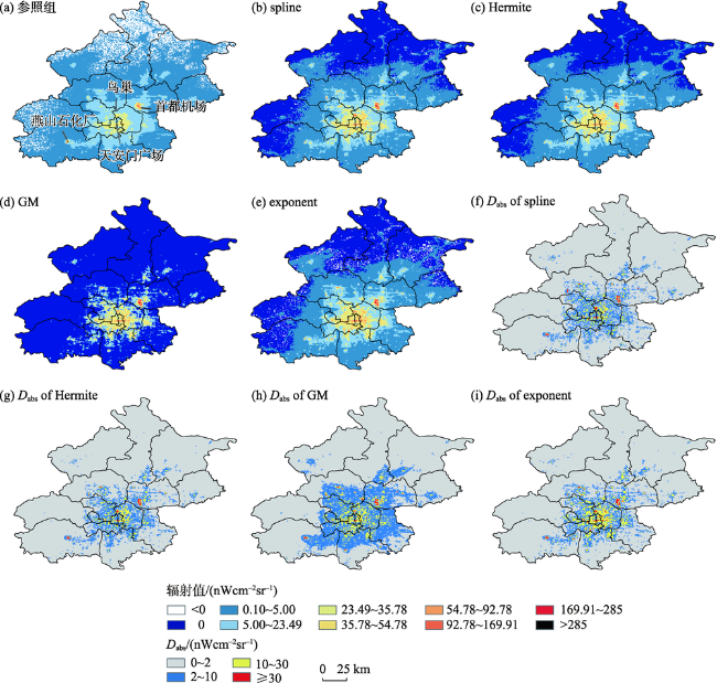
Fig.3 IInterpolation results of June: (a) is Visible Infrared Imaging Radiometer Suite Cloud Mask Stray Light (vcmsl) of June; (b) and (f) are cubic spline interpolation (spline) method's interpolation result and distribution of Dabs, respectively; (c) and (g) are cubic Hermite interpolation (Hermite) method's interpolation result and distribution of Dabs, respectively; (d) and (h) are gray model's (GM) interpolation result and distribution of Dabs, respectively; (e) and (i) are triple exponential smoothing (exponent) method’s interpolation result and distribution of Dabs, respectively图3 6月份插补结果对比图:(a)为6月份“vcmsl”参照值;(b)与(f)分别为三次样条插值(spline)方法的插补结果及其Dabs分级;(c)与(g)分别为三次Hermite插值(Hermite)的插补结果及其Dabs分级;(d)与(h)分别为灰色预测模型(GM)的插补结果及其Dabs分级;(e)与(i)分别为三次指数平滑(exponent)方法的插补结果及其Dabs分级 |
Fig.4 Interpolation results of July: (a) is Visible Infrared Imaging Radiometer Suite Cloud Mask Stray Light (vcmsl) of July; (b) and (f) are cubic spline interpolation (spline) method's interpolation result and distribution of Dabs, respectively; (c) and (g) are cubic Hermite interpolation (Hermite) method's interpolation result and distribution of Dabs, respectively; (d) and (h) are gray model's (GM) interpolation result and distribution of Dabs, respectively; (e) and (i) are triple exponential smoothing (exponent) method's interpolation result and distribution of Dabs, respectively图4 7月份插补结果对比图:(a)为7月份“vcmsl”参照值;(b)与(f)分别为三次样条插值(spline)方法的插补结果及其Dabs分级;(c)与(g)分别为三次Hermite插值(Hermite)的插补结果及其Dabs分级;(d)与(h)分别为灰色预测模型(GM)的插补结果及其Dabs分级;(e)与(i)分别为三次指数平滑(exponent)方法的插补结果及其Dabs分级 |
Tab.2 Classification of absolute difference value表2 差异绝对值分布范围分段统计 |
| 预测月份 | Dabs分级/(nWcm-2sr-1) | 三次样条插值 | 三次Hermite插值 | 灰色预测模型 | 三次指数平滑 | |||||||||
|---|---|---|---|---|---|---|---|---|---|---|---|---|---|---|
| 比例/% | 平均值/ (nWcm-2sr-1) | 比例/% | 平均值/ (nWcm-2sr-1) | 比例/% | 平均值/ (nWcm-2sr-1) | 比例/% | 平均值/ (nWcm-2sr-1) | |||||||
| 5月 | 0~2 | 88.55 | 0.28 | 91.40 | 0.24 | 74.78 | 0.45 | 90.65 | 0.27 | |||||
| 2~10 | 10.04 | 4.41 | 8.05 | 4.09 | 22.18 | 4.49 | 8.66 | 4.09 | ||||||
| 10~30 | 1.30 | 14.54 | 0.52 | 14.56 | 2.99 | 13.86 | 0.62 | 14.28 | ||||||
| ≥30 | 0.11 | 46.19 | 0.03 | 41.03 | 0.05 | 42.37 | 0.07 | 51.18 | ||||||
| ADabs/ (nWcm-2sr-1) | 0.93 | 0.64 | 1.77 | 0.72 | ||||||||||
| 6月 | 0~2 | 87.55 | 0.27 | 90.86 | 0.26 | 75.84 | 0.39 | 89.21 | 0.26 | |||||
| 2~10 | 10.94 | 4.34 | 8.42 | 4.01 | 20.89 | 4.49 | 9.83 | 4.21 | ||||||
| 10~30 | 1.34 | 14.87 | 0.62 | 15.08 | 3.12 | 14.09 | 0.85 | 14.50 | ||||||
| ≥30 | 0.17 | 209.37 | 0.10 | 314.35 | 0.15 | 228.50 | 0.11 | 293.43 | ||||||
| ADabs/ (nWcm-2sr-1) | 1.26 | 0.98 | 2.01 | 1.09 | ||||||||||
| 7月 | 0~2 | 86.05 | 0.26 | 86.93 | 0.24 | 73.92 | 0.39 | 84.45 | 0.24 | |||||
| 2~10 | 11.13 | 4.76 | 10.52 | 4.88 | 21.69 | 4.68 | 10.59 | 4.98 | ||||||
| 10~30 | 2.59 | 14.94 | 2.35 | 14.48 | 4.13 | 14.41 | 4.60 | 15.58 | ||||||
| ≥30 | 0.24 | 83.30 | 0.20 | 82.59 | 0.26 | 67.36 | 0.36 | 63.70 | ||||||
| ADabs/ (nWcm-2sr-1) | 1.34 | 1.23 | 2.08 | 1.68 | ||||||||||
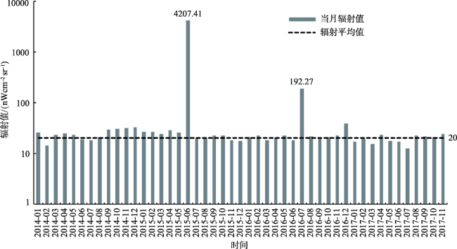
Fig.5 Time series of radiation average surrounding the Yanshan Petrochemical Production Plant (logarithmic scale)图5 燕山石化生产厂附近辐射平均值的时间序列(对数坐标) |
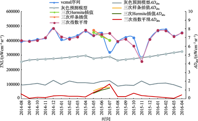
Fig.6 Time series of day/night band (DNB) summation and ADabs from August 2014 to April 2016图6 2014年8月至2016年4月TNL与ADabs的时间序列变化曲线 |
Tab.3 Comparison of the four interpolation methods表3 3种插补方法对比 |
| 三次样条插值 | 三次Hermite插值 | 灰色预测模型 | 三次指数平滑 | |
|---|---|---|---|---|
| 算法思想 | 多项式构造 | 多项式构造 | 一次累加序列拟合 | 原始值的权重累加 |
| 算法适用性 | 仅能插补中间缺失值 | 仅能插补中间缺失值 | 能插补、能预测 | 能插补、能预测 |
| 计算复杂度 | 简单 | 简单 | 简单 | 简单,但重复 |
| 插补精度 | 较高 | 较高 | 较低 | 较高 |
| 计算总时长/s | 9.756 | 9.623 | 9.952 | 1392.927 |
| 平均时长/s | 1.331E-04 | 1.313E-04 | 1.356E-04 | 1.900E-02 |
| 算法优点 | ① 不要求数据符合特定分布 ② 插值综合前后数据 ③ 运行速度快 ④ 插补精度高 | ① 不要求数据符合特定分布 ② 插值综合前后数据 ③ 运行速度快 ④ 插补精度高 ⑤ 不会出现异常值 | ① 不要求数据符合特定分布 ② 所需时序短,只需单侧有值 ③ 运行速度快 ④ 可用于预测 | ① 不要求数据符合特定分布,适用于周期波动非线性序列 ② 所需时序短,只需单侧有值 ③ 可用于预测 ④ 插补精度高 |
| 算法缺点 | ① 数据长度要求高,且要求两侧均有值 ② 容易受异常值影响 ③ 不可用于预测 | ① 数据长度要求高,且要求两侧均有值 ② 容易受异常值影响 ③ 不可用于预测 | ① 不可直接用于非负时间序列预测 ② 插补有效值空间范围小 | ① 运行速度较慢 |
The authors have declared that no competing interests exist.
| [1] |
[
|
| [2] |
[
|
| [3] |
[
|
| [4] |
[
|
| [5] |
[
|
| [6] |
[
|
| [7] |
[
|
| [8] |
[
|
| [9] |
[
|
| [10] |
[
|
| [11] |
[
|
| [12] |
[
|
| [13] |
[
|
| [14] |
[
|
| [15] |
[
|
| [16] |
[
|
| [17] |
[
|
| [18] |
[
|
| [19] |
[
|
| [20] |
[
|
| [21] |
[
|
| [22] |
|
| [23] |
|
| [24] |
|
| [25] |
|
| [26] |
|
| [27] |
|
| [28] |
|
| [29] |
|
| [30] |
|
| [31] |
|
| [32] |
|
| [33] |
|
| [34] |
|
| [35] |
|
| [36] |
|
| [37] |
|
| [38] |
|
| [39] |
|
| [40] |
|
| [41] |
|
/
| 〈 |
|
〉 |
