彭俊 , 董治宝
, 董治宝
PENG Jun, DONG Zhibao
版权声明: 2016 地理科学进展 《地理科学进展》杂志 版权所有
基金资助:
作者简介:
作者简介:彭俊(1987-),男,湖北红安人,博士生,主要从事释光年代学与气候变化研究,E-mail: pengjun10@mails.ucas.ac.cn。
展开
摘要
光释光(OSL)年代学模型是基于数理统计学的一类概率密度模型,它根据特定的假设条件对样品等效剂量(De)分布进行数学解释,由此估计具有不同沉积历史或者能够代表样品实际埋藏年龄的De组分。年龄模型参数估计常通过极大似然估计(MLE)算法实现,本文尝试了切片采样算法在年龄模型参数优化中的应用。切片采样属于一种马尔科夫链蒙特卡罗采样(MCMC)算法,能根据测量数据与模型的联合似然函数进行随机采样,由此获得参数的采样分布。本文编写了实现年龄模型切片采样算法的应用程序,并使用模拟及实测De数据验证了该算法估计的可靠性。相对于MLE算法,MCMC算法具有对参数初值依赖性低、误差估计更准确的特点,切片采样算法提供了实现释光年龄模型参数估计的一种新方法。
关键词:
Abstract
In Optically Stimulated Luminescence (OSL) dating, statistical age models used for equivalent dose (De) determination are probabilistic models constructed according to mathematical statistics. They are applied to distinguish De populations that are sedimentologically different or to determine a De value that represents the burial dose of a sample. Maximum likelihood estimation (MLE) method is routinely used to optimize parameters of an age model. In the present study, we used the Slice sampling algorithm to determine the parameters of age models. Slice sampling is a Markov chain Monte Carlo (MCMC) sampling method, which enables the sampling distributions of parameters to be obtained from the joint likelihood function that is determined by observations and the specified model. This study applied easily implemented and openly accessible numeric routines to performing the algorithm. We used artificial and measured datasets to check the reliability of the estimates. MCMC method is insensitive to the parameters’ initial states, and the standard errors (or confidence intervals) of parameters assessed using this method are more reliable compared to those based on the Fisher information matrix constructed through numerical differentiation. Our results indicate that the Slice sampling method provides an alternative for age model optimization. Slice sampling method generates an informative estimation for the results of MLE method in age model application.
Keywords:
单片再生剂量法(SAR)(Murray et al, 2000)对样品不同单片的测量可获得一系列De值及其误差估计。自然样品的De分布常表现出一定的分散性,这与样品颗粒的侵蚀、搬运、沉积历史与埋藏环境有关。导致样品De分散的不确定性因素包括内部和外部误差(Duller, 2008),前者主要来源于实验操作、数据分析处理及仪器精度,包括光子计数统计不确定性、曲线拟合误差、仪器可重复率、人工贝塔源辐射剂量率的均一程度、实验室与自然条件下加热与辐射过程的差异、样品不同颗粒释光特性的差异等;后者指样品在搬运与埋藏过程中不同颗粒吸收辐射剂量的变化与不确定性,如埋藏前晒退程度不同造成不同颗粒残余剂量的差异、埋藏环境中不同颗粒贝塔剂量率的空间差异、不同埋藏历史与年龄的颗粒发生混合等(Thomsen et al, 2007)。这些都是可能造成自然沉积样品(尤其是水成沉积物) De值异常分散的原因,即使测量采用的不是单颗粒技术而是包含几十到上百粒样品的多颗粒单片(Rodnight et al, 2006; Schmidt et al, 2012; Keen-Zebert et al, 2013)。对于De分布分散的样品,一般不能通过均值计算其埋藏剂量(Galbraith et al, 2012)。
有限组分混合年龄模型(FMM)(Galbraith et al, 1990; Roberts et al, 2000)和最小年龄模型(MAM)(Van der Touw et al, 1997; Galbraith et al, 1999)是两种应用广泛的统计学年龄模型,其模型参数常使用MLE算法来优化。但MLE算法的缺点在于优化结果对参数的初值敏感,模型容易陷入局部最优解。对于多参数模型或高噪声观测数据,MLE算法需比较以不同初值初始化的优化结果才能确定模型的全局最优解。此外,MLE算法不能直接估计参数的标准误差,参数误差常通过费歇尔信息矩阵来估计。对于样本量无限大的样本数据,假定模型的对数似然函数为二次型形式,则模型参数的方差—协方差矩阵等价于费歇尔信息矩阵的逆矩阵(Neale et al, 1997),对该逆矩阵主对角元素取平方根即可得到参数标准误差的近似估计。然而一般统计模型的对数似然函数(包括本文分析的年龄模型)很难满足二次型形式,造成基于信息矩阵的参数误差估计不准确。近年来,随机采样算法在释光年代学数据分析中得到广泛应用,Rhodes等(2003)使用贝叶斯方法将样品地层序列与释光年代数据并入沉积模型,并使用MCMC算法对年代序列进行了校正;Sivia等(2004)应用MCMC算法实现了基于下限De误差的混合分布模型参数估计;Duller(2007)使用蒙特卡罗算法模拟了De计算的误差传递过程;Huntriss(2008)使用MCMC采样技术分析了联合线性剂量模型De分布与多温度预热评估模型初始温度分布;Zink(2013)使用MCMC技术分析了样品沉积过程中多种因素对埋藏剂量分布的影响;Peng等(2014)使用MCMC算法改进了SAR法De误差估计方法,提高了De估计的精度;彭俊等(2015)使用蒙特卡罗算法模拟了剂量率计算过程中多变量耦合误差的传递过程。本文简要介绍了一种MCMC算法(切片采样)的随机采样原理,尝试应用该算法估计释光年龄模型的参数及误差,旨在克服MLE算法对模型参数初值敏感及误差估计不准确的缺点,编写了执行MCMC随机采样算法的程序软件,并根据模拟及实测De数据验证了该算法参数估计的可靠性。
FMM模型常用来估计呈多峰分布的De数据不同组分的特征De值,微尺度上辐射剂量率的不均一是造成De分布呈多峰现象的原因之一,临近放射性活动强的矿物(如钾长石和锆石)的颗粒剂量率高于平均水平,而接近低放射性活动物质(如碳酸钙结核)的颗粒剂量率低于平均水平,由此造成同一沉积层位的样品不同颗粒吸收的累积辐射剂量的空间差异。此外,生物沿垂直地层上下移动造成具有不同年龄的颗粒发生混合(Bateman et al, 2007),也可能造成De数据呈多峰分布。假定单组分De值服从正态分布(Galbraith, 2003),则k组分FMM模型的对数联合似然函数可表示为:
式(1)中:zi与s(zi)分别表示第i个De值及其测量误差;yi与xi分别表示第i个自然对数De值及其相对误差;pj和μj分别表示第j个De组分的比重及特征De值(自然对数尺度);fij表示第i个De值对第j个De组分似然函数的贡献;σ为De分布的已知附加误差(相对误差尺度),表示SAR法De误差估计中被忽略的误差来源,包括仪器可重复性误差、非泊松分布的光子计数统计误差、热转移效应误差以及人工贝塔源辐射剂量率误差等;LFMM表示FMM模型的对数似然值;n表示De值的数目。模型组分数k可通过贝叶斯信息准则(Schwarz, 1978)估计,关于贝叶斯信息准则在模型选择中的应用可参考Peng等(2014)。
在此有必要解释一下模型参数估计之前对观测数据(De及其误差)作自然对数转换的必要性。因为通常SAR法估计的De绝对误差随De增加而增大,造成实测De数据服从概率密度曲线呈正偏态的对数正态分布,对观测数据求自然对数(出现负De值的年轻样品除外)可将其转换为正态De分布(对数正态分布变量的对数值服从正态分布),这有利于消除正偏态数据结构对年龄模型优化结果可靠性的影响(因为年龄模型要求单组份De服从正态分布)。而将De的绝对标准误差转化为相对标准误差的原因主要有两点:(1) 相对标准误差受De值变化的影响较小(Arnold et al, 2009),为比较同一样品不同测片De误差及不同样品不同测片De误差提供了更合理的标准;(2) 对于同一变量,其相对误差近似等于其自然对数值的绝对误差(Galbraith et al, 2012),因此在对De值取自然对数后,只有相应地将De值的绝对误差变为相对误差才能维持原始数据中De值与误差值之间的幅度关系。
样品颗粒埋藏前晒退不完全也是造成De分布分散的原因之一,用于晒退不完全沉积样品De估计的统计方法有多种,Olley等(1998)使用De分布最低5%分位数内的单片De均值来估计样品De;Lepper等(2002)使用正态分布函数拟合De分布直方图的前缘区域,将拟合获得的正态分布函数中二阶导数为零的点确定为样品De;Zhang等(2003)通过比较经感量校正的再生OSL信号与自然OSL信号的相对标准偏差来选择晒退完全的单片De,并将其均值作为样品De;Thomsen等(2007)将呈升序排列的De数据“内部”与“外部”测量误差比值为整数1的单片De均值作为样品De;Pietsch(2009)使用正态分布函数拟合De分布多峰概率密度曲线的最前峰,将拟合得到的正态分布函数均值作为样品De。但这些选取晒退完全单片De组分的方法都属于经验性方法,缺乏严格的数理统计学理论作为依据,估计的样品De可靠性在很大程度依赖于分析所用的样品数据。相比之下,MAM模型是应用最广泛的分析晒退不完全De分布的统计学模型,它的建立以严格数理统计学准则为基础。该模型分3参数(MAM3)与4参数(MAM4)两种类型,MAM4模型对De数据内在结构(如De分布的离散度、De值的数目、De数据的相对误差等)的要求较高,数值稳定性差,因而应用较少。相比之下,MAM3普适性强,数值稳定性高,被广泛用于不同类型沉积样品的De估计(Schmidt et al, 2012; Kunz et al, 2013; Ou et al, 2015)。假设样品颗粒因埋藏前被晒退到不同程度而造成晒退完全与不完全的颗粒共存,由此样品De分布可看作由完全晒退组分和未完全晒退组分按一定比例形成的混合概率密度分布函数,则MAM3模型的对数联合似然函数可表示为:
式(2)中:γ0与σ0为模型优化过程中间环节的代用参数,并无实际物理意义;yi与xi分别表示第i个对数De值及其相对误差(与式(1)相同);fi1与fi2分别第i个De值对晒退完全组分与非完全组分似然函数的贡献;模型的3个待估参数为p、γ、σ,其中p表示晒退完全De组分的比重,γ代表晒退完全De组分的特征De值(自然对数尺度),σ为表征未完全晒退组分De离散程度的附加误差(相对误差尺度);Φ(x)表示标准正态分布累积函数,LMAM3表示MAM3模型的对数似然值。
Metropolis-Hasting和 Gibbs是常见的两种随机采样算法,这两种算法对概率密度模型的适应性因具体模型而异。Metropolis-Hasting算法需先指定一个便于随机数生成的“建议”分布函数,然后以“接受—拒绝”方式决定是否接受新生成的随机数。“建议”分布与目标分布函数越相似,采样效果越好。但对于复杂分布函数,如何选择“建议”分布函数并非易事,它直接影响到目标分布函数样本的质量。在Gibbs采样中,模型不同参数通过条件概率密度分布发生联系,随机变量出现(生成)的概率由其满条件分布和其余变量的当前值共同决定,通过依次轮流的方式实现多参数样本更新(Gelman et al, 2013; Lunn et al, 2013)。Gibbs算法的缺点在于需先确定参数的满条件分布,满条件分布为标准分布函数(如指数、正态分布等)的参数可直接采样,但满条件分布复杂的变量需使用其他算法(如Metropolis-Hasting、切片采样算法等)获得其采样分布。
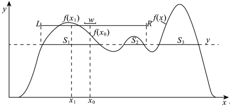
切片采样(Neal, 2003)为一种广义的Gibbs采样算法,属于附加变量采样技术。Neal(2003)指出,单变量概率函数的采样分布可通过对其概率密度曲线下方区域对应变量值的随机均匀采样获得。切片采样算法在生成密度函数f(x)的随机变量x1之前,需引入附加变量y,其生成随机变量的方法通过如下迭代步骤实现:①给定初值x0,然后从区间(0, f(x0))中随机均匀地生成附加变量y,切片S对应的横轴x值集合为{x; f(x)>y};②确定以x0为扩张基点的采样区间I=(L, R),该区间应尽可能的覆盖水平切片S的绝大部分;③从采样区间I中随机均匀地生成新变量x1。图1为单变量切片采样算法示意图,图中由均匀分布随机变量y确定的水平切片S被概率密度函数f(x)分割为小切片S1、S2、S3,与切片S对应的横轴所有x值满足f(x)>y。以x0为基点的样本区间以w为步长持续增加宽度,直到该样本区间的两端扩张到切片S以外的区域,然后从扩张后的样本区间I=(L,R)中随机均匀地生成新变量x1。
图1 单变量概率密度函数的切片采样算法实现示意图
Fig.1 Single-variable Slice sampling by simulating a sample from the region under its density function f(x)
切片采样算法最棘手环节在于如何确定采样区间I的边界使其尽可能的覆盖切片S。若能确定概率密度函数f(x)反函数f -1(x)的解析式,便能精确界定采样区间I的边界。但很多复杂概率密度模型不能被反解,且函数f(x)的起伏变化容易对水平切片S形成切割作用,使得区间I呈现多重边界因而很难逐一界定。为此,Neal(2003)提出了名为“Stepping out”和“Shrinkage”的方法来确定区间I边界。首先以x0为基点定义宽度为w的微型水平区间I,然后以w为步长重复扩张该区间,直到区间I的两端超出水平切片S的范围,即f(x)≤y。由于采样区间I=(L,R)对应的横轴x值不一定全部满足f(x)>y,所以若新生成的随机数x1位于切片外部,则需要收缩区间I两端,然后再次生成x1,重复此过程直到生成的x1满足f(x1)>y为止,随着不满足条件的随机变量不断被拒绝及区间I的逐步收缩,生成符合条件的随机数x1的概率逐渐增加。
通过类似于Gibbs算法对不同变量轮流依次采样的方式(表1),将每个参数的分布函数当作条件性依赖于其他参数当前值的单变量概率模型,则上述单变量切片采样算法可直接推广应用于多参数概率密度模型采样。本文编写了进行MAM与FMM模型切片采样的开源R软件程序(Peng et al, 2013; 彭俊等, 2016) (http://CRAN.R-project.org/package=numOSL)。由于MCMC采样过程消耗内存且费时,为提高运算效率,本文核心程序使用Fortran语言编写,通过接口方式在R软件环境下调用。获得模型参数分布之后,便可根据中心极限定理来估计参数的期望值,并计算标准偏差、众数、百分位数等统计量。需要注意的是,由于模型分析时观测数据(De)被转换到自然对数尺度,因此算法运行结束后需将De的采样分布转化到非自然对数尺度才能进行样本统计分析。此外,考虑到交换FMM模型不同组分参数位置不影响模型的似然函数值,例如,将FMM第1组分参数(p1, μ1)与第2组分参数(p2, μ2)交换位置并不影响对数似然函数LFMM的值,混合模型组分参数的这种特性称为“标签置换”,该效应可能会引起随机参数在样本链中的位置发生置换变动。本文程序通过对FMM模型生成的随机样本作μ1<μ2<…<μk的定向排序来减小“标签置换”效应对参数估计结果的影响。
表1 多变量切片采样算法流程
Tab.1 A general procedure for applying the Slice sampling method to sampling from a multivariable model
| 输入:概率模型,迭代总次数nsim,初始参数状态X0,模型参数总 数N; 输出:随机采样样本及参数估计结果 |
|---|
| 1. 分配用于随机样本储存的数据矩阵(chain):chain=matrix(nrow=nsim, ncol=N); |
| 2. 通过如下迭代方式对参数轮流更新: do i=1, nsim do j=1, N 根据切片采样算法以条件概率P(Xj/X0[-j])生成随机 变量Xj X0[j] = Xj chain[i,j] = Xj end do end do 3. 根据随机样本数据chain 进行参数估计 |
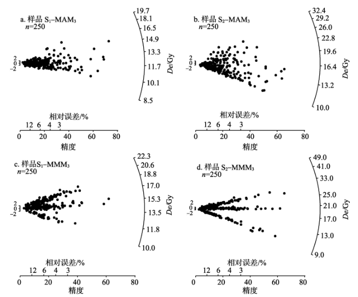
SAR测量的De值的绝对误差与其大小有关,较大De值的误差也较大(Galbraith et al, 2012)。然而,De值的相对误差可认为独立于De值变化(Arnold et al, 2009)。本文以一组实测De数据的误差结构为参照,从参数值已知的年龄模型中生成随机De分布,旨在使模拟生成的随机De数据的误差结构更接近实测SAR De的误差结构。所用的实测De数据的相对误差近似服从均值为7.5%,标准偏差为5%的对数正态分布(Arnold et al, 2009)。随机De数据按如下方式生成:①确定模型参数及随机De值的初始状态y0;②生成服从上述对数正态分布的De相对误差x;③使用单变量切片采样算法从参数已知的年龄模型中生成随机De值y(对数尺度),y条件地依赖于y0与x;④将对数尺度De值y及其相对误差x转换为自然尺度De值z及绝对误差s(z),即,z=exp(y),s(z)=exp(y)·x。本文根据上述方法使用列于表2-3中的已知参数从不同年龄模型(MAM3和FMM3)中模拟生成随机De数据,对每个模型生成两组离散程度不同的De分布,分别命名为S1-MAM3、S2-MAM3、S1-FMM3、S2-FMM3。对于每组已知参数,先模拟生成10000个随机De值(含De误差),然后舍弃前7500个数据以降低De初始状态y0对随机De分布的影响(“Burn-in”程序),最后从剩余的2500个数据中每10个取1个以降低随机De值间的自相关程度(“Thinning”程序),每组得到250个De数据,由此获得的4组模拟样品De分布见图2。
图2 根据已知模型参数模拟生成样品的De分布
Fig.2 De distributions for simulated samples using age models with known parameters
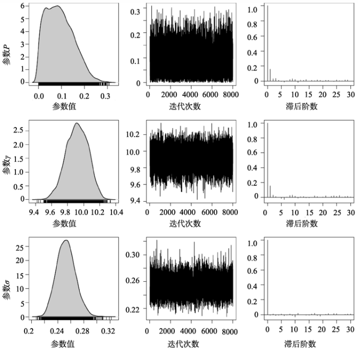
本文在应用切片采样算法估计模拟与实测样品De数据的模型参数时,MCMC算法采样总数均为50000次,舍弃前10000个样本值(“Burn-in”数为10000),然后从剩余样本中每5次迭代取一个样本(“Thinning”数为5),剩余8000个样本用于模型参数估计。模拟样品De数据的MAM3与FMM3模型参数估计结果分别见表2-3,结果表明根据MCMC与MLE算法估计的模型参数值均与实际值是一致的,说明基于切片采样算法的年龄模型参数估计结果是可靠的。图3为使用参数p=0.1、γ=10、σ=0.25生成的随机De分布(模拟样品S1-MAM3)的MAM3模型MCMC算法采样结果,图中第1列为参数的密度分布图,第2列为随机样本随迭代次数变化图,第3列为参数自相关系数变化图。从图中可以看出,随机样本具有良好的混合特性,参数的自相关程度都很低,表明MCMC采样算法收敛到了模型参数的期望分布。此外,图3中MAM3模型参数p的采样分布呈正偏态,MLE算法估计的p值为0.08±0.09,由此根据正态近似法(即value±1.96σ,value表示参数点估计,σ为参数标准偏差)计算的参数p的95%置信区间为(-0.10, 0.25),该区间下限小于零而不符合实际,而根据MCMC算法获得的随机样本分布计算的p值95%置信区间为(0.005, 0.22),可见当参数呈偏态分布时,由正态近似法获得的对称性置信区间不可靠(Galbraith et al, 2012)。
表2 根据已知模型参数生成的De数据的MAM3参数估计
Tab.2 Estimates of MAM3 obtained from De distributions simulated using known parameters
| 样品名称 | 实际参数 | MCMC算法参数估计 | MLE算法参数估计 |
|---|---|---|---|
| S1-MAM3 | p=0.1 | p=0.09±0.06 (0.005, 0.22) | p=0.08±0.09 (-0.10, 0.25) |
| γ=10 | γ=9.92±0.13 (9.64, 10.17) | γ=9.92±0.19 (9.54, 10.29) | |
| σ=0.25 | σ=0.25±0.01 (0.23, 0.28) | σ=0.25±0.01 (0.22, 0.28) | |
| S2-MAM3 | p=0.3 | p=0.20±0.04 (0.12, 0.28) | p=0.20±0.04 (0.12, 0.28) |
| γ=10 | γ=9.82±0.08 (9.66, 9.98) | γ=9.83±0.08 (9.68, 9.98) | |
| σ=0.5 | σ=0.54±0.03 (0.48, 0.60) | σ=0.54±0.03 (0.48, 0.59) |
表3 根据已知模型参数生成的De数据的FMM3参数估计
Tab.3 Estimates of FMM3 obtained from De distributions simulated using known parameters
| 样品名称 | 实际参数 | MCMC算法参数估计 | MLE算法参数估计 |
|---|---|---|---|
| S1-FMM3 | p1=0.1; μ1=10 | p1=0.12±0.02 (0.08, 0.17); μ1=10.06±0.11 (9.85, 10.28) | p1=0.12±0.02 (0.08, 0.16); μ1=10.04±0.11 (9.83, 10.26) |
| p2=0.5; μ2=15 | p2=0.47±0.03 (0.40, 0.53); μ2=15.08±0.07 (14.94, 15.23) | p2=0.47±0.03 (0.41, 0.54); μ2=15.08±0.07 (14.94, 15.22) | |
| p3=0.4; μ3=20 | p3=0.41±0.03 (0.35, 0.47); μ3=20.10±0.11 (19.89, 20.32) | p3=0.41±0.03 (0.34, 0.47); μ3=20.10±0.11 (19.89, 20.32) | |
| S2-FMM3 | p1=0.3; μ1=10 | p1=0.27±0.03 (0.22, 0.33); μ1=10.07±0.06 (9.97, 10.18) | p1=0.27±0.03 (0.21, 0.33); μ1=10.07±0.06 (9.96, 10.18) |
| p2=0.35; μ2=20 | p2=0.41±0.03 (0.35, 0.47); μ2=20.12±0.09 (19.94, 20.30) | p2=0.41±0.03 (0.35, 0.48); μ2=20.12±0.09 (19.94, 20.30) | |
| p3=0.35; μ3=30 | p3=0.32±0.03 (0.26, 0.38); μ3=29.95±0.16 (29.64, 30.26) | p3=0.32±0.03 (0.26, 0.38); μ3=29.95±0.16 (29.64, 30.26) |
图3 模拟样品S1-MAM3De数据的MAM3模型MCMC算法采样结果
Fig.3 MCMC output of MAM3 using simulated De values from sample S1-MAM3
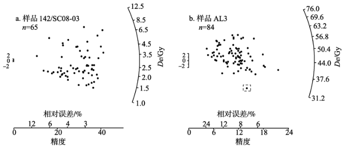
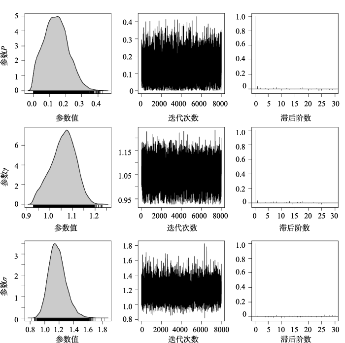
需要注意的是,验证切片采样算法的实用性时,需考虑到模拟数据与实测数据之间的差异。因为尽管以上模拟样品De数据的随机生成过程考虑了实测样品De分布的误差结构,但仅能代表理想状态下的De分布。自然沉积环境中样品不同颗粒辐射剂量率的空间差异、晒退程度差异、不同沉积层位颗粒混合等增加了实测De数据的噪声水平,造成实测De分布复杂而分散。此外,上述每组模拟数据多达250个De值因而包含了丰富的信息量,这有利于提高模型采样过程的稳定性,但实验室实测样品单片De数通常在50以内(一般不超过100)。为此,本文使用两个实测水成沉积样品(142/SC08-03 和 AL3)的De数据对MCMC算法可靠性作进一步验证(图4)。样品142/SC08-03为来自南非东部内陆的河流沉积物,共测量65个De值(Keen-Zebert et al, 2013),样品AL3为来自南美安第斯山脉的冲积扇沉积物,共测量84个De值(Schmidt et al, 2012)。本文在实测数据相对误差的基础上并入10%的附加误差来表示De误差估计中被忽略的误差来源,以免De误差被低估(Galbraith et al, 2005)。由于年龄模型对含异常De值的观测数据敏感,本文在数据分析之前移除了实测De数据AL3中的一个异常值(如图4b虚线方框所示),然后使用MCMC和MLE算法分析了两组数据并对结果进行了比较(表4-5)。对比结果表明,两种算法的参数估计结果很一致。图5为样品142/SC08-03的MAM3模型MCMC采样结果,参数p同样呈明显正偏态分布,MLE算法估计的p值为0.14±0.08,由此根据正态近似法估计的95%置信区间为(-0.02, 0.30),而根据MCMC算法采样分布计算的p值95%置信区间为(0.01, 0.29),后者更合理。样品AL3的MAM3模型MCMC分析结果中参数p结果类似,MLE算法结合正态近似法估计的95%置信区间为(-0.21, 0.60),MCMC算法估计的p值95%置信区间为(0.01, 0.51)。
图4 实测样品142/SC08-03与AL3的De分布
Fig.4 De distributions for measured samples 142/SC08-03 and AL3
图5 实测样品142/SC08-03 De数据的MAM3模型MCMC算法采样结果
Fig.5 MCMC output of MAM3 using measured De values from sample 142/SC08-03
表4 实测De数据的MAM3模型参数估计
Tab.4 Estimates of MAM3 obtained using measured De distributions
| 样品名称 | MCMC算法参数估计 | MLE算法参数估计 |
|---|---|---|
| 142/SC08-03 | p=0.14±0.07 (0.01, 0.29) | p=0.14±0.08 (-0.02, 0.30) |
| γ=1.06±0.05 (0.95, 1.15) | γ=1.07±0.05 (0.97, 1.18) | |
| σ=1.18±0.12 (0.97, 1.44) | σ=1.15±0.11 (0.92, 1.37) | |
| L=-59.34 | L=-59.26 | |
| AL3 | p=0.22±0.14 (0.01, 0.51) | p=0.20±0.21 (-0.21, 0.60) |
| γ=40.56±1.90 (36.78, 44.10) | γ=40.49±2.58 (35.44, 45.54) | |
| σ=0.41±0.05 (0.32, 0.52) | σ=0.39±0.05 (0.30, 0.48) | |
| L=-9.53 | L=-9.45 |
表5 实测De数据的FMM模型参数估计
Tab.5 Estimates of FMM obtained using measured De distributions
| 样品名称 | MCMC算法参数估计 | MLE算法参数估计 |
|---|---|---|
| 142/SC08-03 | p1=0.30±0.05 (0.21, 0.40); μ1=1.15±0.03 (1.09, 1.21) | p1=0.30±0.06 (0.19, 0.42) ; μ1=1.14±0.03 (1.08, 1.20) |
| p2=0.35±0.05 (0.25, 0.45); μ2=1.94±0.05 (1.86, 2.03) | p2=0.37±0.06 (0.25, 0.49) ; μ2=1.94±0.04 (1.85, 2.02) | |
| p3=0.22±0.05 (0.13, 0.31); μ3=4.22±0.14 (3.95, 4.51) | p3=0.20±0.05 (0.10, 0.30) ; μ3=4.19±0.14 (3.93, 4.46); | |
| p4=0.13±0.04 (0.06, 0.23); μ4=9.66±0.47 (8.82, 10.65) | p4=0.12±0.04 (0.04, 0.20); μ4=9.54±0.42 (8.72, 10.35) | |
| L=-97.82 | L=-97.62 | |
| AL3 | p1=0.39±0.11 (0.18, 0.61); μ1=41.31±1.73 (37.69, 44.55) | p1=0.39±0.13 (0.14, 0.65); μ1=41.23±1.77 (37.77, 44.69) |
| p2=0.38±0.10 (0.17, 0.58); μ2=52.91±3.42 (47.08, 60.79) | p2=0.40±0.12 (0.15, 0.64); μ2=53.01±3.08 (46.97, 59.05) | |
| p3=0.23±0.06 (0.12, 0.36); μ3=79.01±4.41 (70.86, 88.12) | p3=0.21±0.06 (0.10, 0.32); μ3=79.72±4.14 (71.60, 87.83) | |
| L=-6.83 | L=-6.74 |
通过给定参数的初始状态(类似于优化问题中的参数初值),MCMC算法以随机游走的方式从概率密度模型采样,采样器能否经过多次迭代后“忘记”初始状态并收敛到模型参数的平稳分布是进行参数估计的前提。用于诊断马氏链是否收敛的方法有多种(Plummer et al, 2006; Lunn et al, 2013),最简单的方法是观察随机样本值随迭代次数的变化,均匀混合的随机样本可在参数状态空间上下自由移动(如图3与图5中第2列)。若随机样本随迭代次数呈阶梯步状式的大幅震荡变化,则说明样本混合不均匀,算法可能未收敛。通过随机样本的自相关系数也可以检验MCMC算法的收敛性:样本的自相关程度越低(如图3和图5中第3列),说明随机样本混合特性越好,算法收敛越快。通常在使用随机样本进行统计推断之前,先要对样本数据进行“修剪”,这是因为随机样本的初始部分可能未收敛到参数的平稳分布而需将其删除(称为“Burn-in”程序),而为降低随机序列的自相关程度需从每数个样本中取1个(称为“Thinning”程序)。若“修剪”后随机样本的混合特性仍很差或自相关度仍很高,则说明算法未收敛。
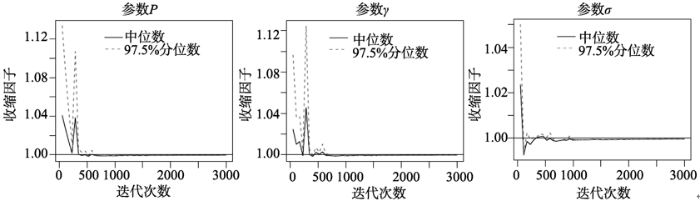
Gelman-Rubin 收敛诊断法 (Gelman et al, 1992)是应用最广泛的马氏链收敛诊断法,它对同一组观测数据使用不同初始状态随机采样由此获得多组平行马氏链,然后根据收缩因子(Shrink factor)来测量链内与链间方差的差异(类似于方差分析),若收缩因子小于等于1则说明算法收敛。本文设置5组不同初始状态,应用MAM3模型分析了实测样品AL3的De数据,并使用Gelman-Rubin 收敛诊断R软件程序包coda(Plummer et al, 2006)分析了根据切片采样法生成的5组平行马氏链,结果见图6。在最初的300次迭代中,各参数(p、γ、σ)的收缩因子都出现大幅度震荡,但均在1000次迭代内降到1以下,说明随机生成的马氏链收敛到了MAM3模型的平稳分布。
图6 应用MAM3模型分析样品AL3 De数据的Gelman-Rubin 收敛诊断结果
Fig.6 Gelman-Rubin diagnostic plots for MCMC output of MAM3 using De values of sample AL3
在本文所有De数据(包括模拟和实测样品)的MCMC算法分析中,没有出现必须调整参数初始状态才能顺利完成随机采样的情况,而是一直使用程序默认设置的初始参数。此外,应用差异很大的初始状态于同一组De数据获得的马氏链的参数估计结果完全一致,表明本文所采用的切片采样器对参数的初始状态不敏感,能够在有限次迭代内收敛到模型的平稳分布(全局最优解)。而MLE算法在不同初始化条件下的参数估计不尽相同,Rex Galbraith提出使用观测数据范围内等距间隔的De分位值作为FMM模型特征De初值,这种初始化方式在大多数情况下均有效,但对于高噪声De数据,其优化参数可能仅收敛到局部极值,因此应用MLE算法时有必要使用基于试错法的高强度、多初值反复优化的方式来确定模型的全局最优解。本文建议通过对同一组De数据进行不同算法结果的比较分析来确定合理的参数估计,以免造成对De分布的错误解释。
模拟样品De数据的分析结果表明切片采样算法的参数估计与模型实际参数是一致的,而两种不同算法对实测样品De数据的分析进一步验证了MCMC算法估计结果的可靠性。MLE算法常使用费歇尔信息矩阵近似代替方差—协方差矩阵来估计模型参数的误差,信息矩阵可通过对参数求偏导获得,复杂模型的信息矩阵常采用有限差分逼近来计算,逆信息矩阵主对角元素的平方根可近似作为参数标准误差。但基于信息矩阵的参数不确定性估计要求模型似然函数为二次型形式(Neale et al, 1997),而一般似然模型并不满足该要求。而在MCMC算法中,直接可靠的误差估计可通过计算采样分布的标准偏差实现(Galbraith et al, 2012)。此外,根据中心极限定理,当观测变量的采样分布趋于服从正态分布时,根据正态分布的对称性可使用正态近似法计算参数的置信区间,例如,假定参数value的标准误差为σ,则对应的95%置信区间的近似估计为(value-1.96σ, value+1.96σ),但若参数的采样分布呈一定的偏度(如图3、图5中MAM3模型的参数p),则通过正态近似法计算的置信区间不可靠。而对于MCMC算法,参数的置信区间可直接根据采样分布计算,显著性水平α对应的100(1-α)%置信区间由采样分布的(α/2)%和(1-α/2)%分位数决定,例如,显著性水平为0.05时参数p的95%置信区间介于p样本分布的2.5%与97.5%分位数之间。
必须指出,正如所有的MCMC算法一样,本文采用的切片采样算法也有自身缺点。模型参数的采样分布通常需要由数万次迭代计算(本文程序默认迭代次数为5万次)获得,随模型复杂度及观测数据的增加,需要越来越长的时间才能完成采样过程。MLE算法在不足1s内便能完成的运算而MCMC算法甚至需要几分钟时间才能完成,这对计算机内存和运算时间都是极大的考验。MCMC算法不能对生成的随机样本充分利用,在本文模型参数估计中的利用率仅为8/50=16%,造成了计算资源浪费。此外,采样算法收敛程度是衡量参数估计结果可靠性的重要指标,所以利用MCMC算法进行参数估计之前,需要对获得的随机样本链进行常规性收敛检验。最后,本文采用的切片采样算法在迭代过程中每个参数都条件依赖于其他参数而依次更新,这可能会增加随机样本的自相关程度并增加“Burn-in”与“Thinning”程序所需的样本量。如何改进算法(如将切片采样算法的参数更新方式由依次更新变为同步更新)从而加快算法收敛速度并提高资源利用率是今后研究的重点。
致谢:感谢Silke Schmidt博士、Helena Rodnight博士、欧先交博士、Amanda Keen-Zebert 博士提供的用于模型验证的实测De数据。
The authors have declared that no competing interests exist.
| [1] |
基于R语言的光释光年代学数据处理程序包numOSL程序设计及应用实例分析 [J].Developing a package numOSL for analyzing optically stimulated luminescence data using the R statistical language and its practical application [J]. |
| [2] |
基于Monte Carlo 方法的释光测年剂量率误差估计 [J].https://doi.org/10.11889/j.0253-3219.2015.hjs.38.070201 Magsci 摘要
在释光年代学上,剂量率代表样品埋藏过程中单位时间内吸收的辐射剂量,其估计直接影响到埋藏年代的可靠性。误差传递公式(Quadratic propagation of uncertainty)常用于剂量率误差估计。由于计算剂量率涉及到众多参数复杂的非线性运算,造成基于误差传递公式的误差估计过程繁琐复杂。本文以粗颗粒石英矿物为例介绍了剂量率计算过程及误差估计方法,使用蒙特卡罗误差传递法(Monte Carlo error propagation)模拟了剂量率计算过程中多参数不确定性耦合误差,编写了执行随机剂量率模拟运算的开源R程序,并通过实测数据展示了该技术的应用。相对于应用误差传递公式法估计剂量率误差,Monte Carlo方法具有直观灵活、简便科学的特点,这种随机策略在分析科学领域具有广泛的适用性。
Determining the error of dose rate estimates on luminescence dating using Monte Carlo approach [J].https://doi.org/10.11889/j.0253-3219.2015.hjs.38.070201 Magsci 摘要
在释光年代学上,剂量率代表样品埋藏过程中单位时间内吸收的辐射剂量,其估计直接影响到埋藏年代的可靠性。误差传递公式(Quadratic propagation of uncertainty)常用于剂量率误差估计。由于计算剂量率涉及到众多参数复杂的非线性运算,造成基于误差传递公式的误差估计过程繁琐复杂。本文以粗颗粒石英矿物为例介绍了剂量率计算过程及误差估计方法,使用蒙特卡罗误差传递法(Monte Carlo error propagation)模拟了剂量率计算过程中多参数不确定性耦合误差,编写了执行随机剂量率模拟运算的开源R程序,并通过实测数据展示了该技术的应用。相对于应用误差传递公式法估计剂量率误差,Monte Carlo方法具有直观灵活、简便科学的特点,这种随机策略在分析科学领域具有广泛的适用性。
|
| [3] |
Stochastic modelling of multi-grain equivalent dose (De) distributions: Implications for OSL dating of sediment mixtures [J].https://doi.org/10.1016/j.quageo.2008.12.001 URL Magsci [本文引用: 3] 摘要
A number of recent optically stimulated luminescence (OSL) studies have cited post-depositional mixing as a dominant source of equivalent dose () scatter across a range of sedimentary environments, including those previously considered ‘best suited’ for OSL dating. The potentially insidious nature of sediment mixing means that this problem may often only be identifiable by careful statistical analysis ofdata sets. This study aims to address some of the important issues associated with the characterisation and statistical treatment of mixeddistributions at the multi-grain scale of analysis, using simulateddata sets produced with a simple stochastic model. Using this Monte Carlo approach we were able to generate theoretical distributions of single-grainvalues, which were then randomly mixed together to simulate multi-grain aliquotdistributions containing a known number of mixing components and known corresponding burial doses. A range of sensitivity tests were undertaken using sediment mixtures with different aged dose components, different numbers of mixing components, and different types of dose component distributions (fully bleached, heterogeneously bleached and significantly overdisperseddistributions). The results of our modelling simulations reveal the inherent problems encountered when dating mixed sedimentary samples with multi-grainestimation techniques. ‘Phantom’ dose components (i.e. discrete dose populations that do not correspond to the original single-grain mixing components) are an inevitable consequence of the ‘averaging’ effects of multi-grainanalysis, and prevent the correct number of mixing components being identified with the finite mixture model (FMM) for all of the multi-grain mixtures tested. Our findings caution against use of the FMM for multi-grain aliquotdata sets, even when the aliquots consist of only a few grains.
|
| [4] |
Detecting post-depositional sediment disturbance in sandy deposits using optical luminescence [J].https://doi.org/10.1016/j.quageo.2006.05.004 URL [本文引用: 1] 摘要
This paper examines sites from Texas and Florida (USA) with independent chronological control to demonstrate the potential effects of varying degrees of bioturbation on OSL. Results show that contemporary soil forming processes clearly impact on the palaeodose ( D e ) replicate distributions which are measured in order to derive an OSL age. Significant levels of scatter and apparently zero dose grains are observed in the upper-most sediments; declining with depth from the surface. D e replicates from undisturbed and fully bleached sediments are unskewed, show low overdispersion (OD) and comparable single grain and single aliquot OSL ages. Bioturbated sediments, however, may show highly skewed multi-model D e distributions with higher OD values, zero dose grains at depth, and significant diffences between single grain and single aliquot results. True burial ages may be derived from minimally bioturbated sediments through the application of statistical analysis such as finite mixture modelling to isolate D e components. However, for significantly bioturbated sediments, the latter approach, even at the single grain level, produces inaccurate ages. In such cases we argue that additional evidence (both dating and contexual) may be required to identify with confidence the burial D e population.
|
| [5] |
Assessing the error on equivalent dose estimates derived from single aliquot regenerative dose measurements. URL 摘要
Measurement of the equivalent dose (De) is central to luminescence dating. Single aliquot methods have been developed in the last 10-15 years, first with the description of methods suitable for feldspars (Duller 1995) and subsequently those applicable to quartz (Murray and Wintle 2000, 2003). Such methods have the advant...
|
| [6] |
Single-grain optical dating of Quaternary sediments: Why aliquot size matters in luminescence dating [J].https://doi.org/10.1111/j.1502-3885.2008.00051.x URL [本文引用: 1] 摘要
Geoffrey A. T. Duller (e-mail: ggd@aber.ac.uk), Institute of Geography and Earth Sciences, Aberystwyth University, Aberystwyth SY23 3DB, Wales, UK
|
| [7] |
A simple homogeneity test for estimates of dose obtained using OSL [J].
In optical dating (and in other dating methods) it is often required to compare age estimates, or equivalent dose estimates, for a number of single grains or aliquots. Typically each estimate has a different and (hopefully) known precision, which needs to be taken into
|
| [8] |
Estimating the component ages in a finite mixture [J].https://doi.org/10.1016/1359-0189(90)90035-V URL [本文引用: 1] 摘要
The calculations are experimentally tested using data obtained from synthetic mixtures of grains, so that the estimates can be compared with known values and also in order to demonstrate the applicability of the method.
|
| [9] |
Statistical aspects of equivalent dose and error calculation and display in OSL dating: An overview and some recommendations [J].https://doi.org/10.1016/j.quageo.2012.04.020 URL [本文引用: 5] 摘要
All Quaternary dating methods involve the measurement of one or more variables to estimate the age of a sample. Each measured quantity has an associated error and uncertainty, and may also be subject to natural variation. We review the statistical estimation of such uncertainties and variation for comparing and interpreting age estimates, with specific reference to the estimation of equivalent dose ( D e ) values in the optically stimulated luminescence (OSL) dating of sediments. We discuss statistical aspects of OSL signal and background estimation, the determination of D e values for multi-grain aliquots and individual mineral grains from the same and different samples, and the extent of variation commonly observed among such estimates. Examples are drawn from geological and archaeological contexts. We discuss the strengths and weaknesses of various graphical methods of displaying multiple, independent estimates of D e , along with statistical tests and models to compare and appropriately combine them. Many of our recommendations are applicable also to the clear presentation of data obtained using other Quaternary dating methods. We encourage the use of models and methods that are based on well established statistical principles and, ideally, are validated by appropriate numerical simulations; and we discourage the adoption of ad hoc methods developed using a particular set of measurement conditions and tested on a limited number of samples, as these may not be applicable more generally. We emphasise that the choice of statistical models should not be made solely on statistical grounds (or arbitrary rules) but should take into account the broader scientific context of each sample and any additional pertinent information.
|
| [10] |
Optical dating of single and multiple grains of quartz from Jinmium rock shelter, northern Australia: Part I, experimental design and statistical models [J].https://doi.org/10.1111/j.1475-4754.1999.tb00987.x URL [本文引用: 1] 摘要
Jinmium rock shelter is famous for the claims made by Fullagar et al. (1996) for the early human colonization and ancient rock art of northern Australia. These claims were based on thermo-luminescence ages obtained for the artefact-bearing quartz sediments that form the floor deposit at the site. In this paper, we outline the background to the optical dating programme at Jinmium, and describe the experimental design and statistical methods used to obtain optical ages from single grains of quartz sand. The results, interpretations, and implications of this dating programme are reported in a companion paper (Roberts et al. 7999, this volume).
|
| [11] |
Error variation in OSL palaeodose estimates from single aliquots of quartz: A factorial experiment [J]. |
| [12] |
|
| [13] |
A Bayesian analysis of luminescence dating[D]. Durham, British:
|
| [14] |
A Bayesian analysis of luminescence dating[D].
|
| [15] |
Late Quaternary floodplain reworking and the preservation of alluvial sedimentary archives in unconfined and confined river valleys in the eastern interior of South Africa [J].https://doi.org/10.1016/j.geomorph.2012.12.004 URL Magsci [本文引用: 2] 摘要
In this study, geomorphological, sedimentological, and geochronological work was conducted on unconfined and confined reaches of three rivers in the eastern interior of South Africa in order to quantify the relative rates of floodplain reworking and alluvial preservation along river courses with variable valley confinement and lithology. Using optically stimulated luminescence (OSL) dating techniques, new chronologies for the Schoonspruit and Mooi River were created and the existing Klip River chronology was expanded. The results suggest that floodplains in both unconfined and confined reaches preserve complex spatial and temporal patterns of alluviation, although differences in boundary conditions lead to variation in the processes and rates of floodplain construction and reworking. On the Klip and Mooi Rivers where local base levels are stable, channels in unconfined reaches rework floodplain sediments through slow lateral migration punctuated by local erosion during avulsion events. On the Schoonspruit where base level has lowered, the channel in the unconfined reach is incised, the floodplain is abandoned, and a large gully has formed. In the confined reaches of all three rivers, the narrow floodplains are reworked by scour and fill activity and limited lateral migration. The OSL results suggest that unconfined reaches preserve relatively continuous alluvial records that extend into the Pleistocene, while the floodplains in the confined reaches preserve relatively discontinuous alluvial records biased toward the late Holocene. The alluvial geochronologic records in these systems preserve signals of changes in local base level controlled by variation in lithology and incision rather than climate change. By defining the processes, rates, and patterns of floodplain reworking in reaches with different degrees of valley confinement and channel incision, the findings contribute to understanding how rivers build, modify, and preserve alluvial sedimentary archives. (C) 2012 Elsevier B.V. All rights reserved.
|
| [16] |
Optically stimulated luminescence dating of young fluvial deposits of the Middle Elbe River Flood Plains using different age models [J].https://doi.org/10.2478/s13386-013-0140-7 URL [本文引用: 1] 摘要
In the last few decades optically stimulated luminescence (OSL) dating has become an important tool in geochronological studies. The great advantage of the method, i.e. dating the depositional age of sediments directly, can be impaired by incomplete bleaching of grains. This can result in a scattered distribution of equivalent doses (D E ), leading to incorrect estimation of the depositional age. Thoroughly tested protocols as well as good data analysis with adequate statistical methods are important to overcome this problem. In this study, samples from young fluvial sand and flood plain deposits from the Elbe River in northern Germany were investigated to compare its depositional ages from different age models with well-known historical dates. Coarse grain quartz (100–200 μm and 150–250 μm) and polymineral fine grains (4–11 μm) were date
|
| [17] |
An objective methodology for dose distribution analysis [J].https://doi.org/10.1093/oxfordjournals.rpd.a005999 URL PMID: 12382765 摘要
The advent of single aliquot optically stimulated luminescence (OSL) techniques along with parallel equipment advances have made it possible and practical to obtain statistically meaningful quantities of equivalent dose (De) data from individual samples. Now that hundreds of dose determinations can be made for one sample De distributions may be scrutinised, leading to the problem of how to make unbiased comparisons among distributions, and how to decide objectively which dose is representative of the age of the deposit. In this paper, an objective analytical method is presented for treating dose distributions, including a mathematically rigorous means of determining a representative equivalent dose and a statistical definition of its corresponding uncertainty. This analytical method has been applied to Holocene aeolian and fluvial quartz sands from Central Oklahoma. The results are compared to equivalent doses determined via other proposed analytical procedures.
|
| [18] |
The BUGS book: A practical introduction to bayesian analysis [M]. |
| [19] |
Luminescence dating of quartz using an improved single-aliquot regenerative-dose protocol [J].https://doi.org/10.1016/S1350-4487(99)00253-X URL [本文引用: 1] 摘要
Single aliquot protocols are now widely used as a means of measuring the equivalent dose ( D e ) in quartz and feldspar optical stimulated luminescence (OSL) dating of both heated and sedimentary materials. The most recent of these is the single-aliquot regenerative-dose (SAR) protocol, first suggested by Murray and Roberts (Radiation Measurements 29, 503–515, 1998). In this approach, each natural or regenerated dose OSL measurement is corrected for changes in sensitivity using the OSL response to a subsequent test dose (10–20% of D e ). If the sensitivity correction is adequate, then the corrected OSL response should be independent of prior dose and thermal/optical treatment, i.e. there should be no change in the sensitivity-corrected dose–response curve on remeasurement. Here we examine the interpretation of the sensitivity corrected growth curve as a function of dose, and the effect of changing measurement conditions (e.g. preheat temperature, size of test dose, stimulation temperature) on the estimation of D e . The dependence of the dose response on prior treatment is tested explicitly, and the significance of thermal transfer discussed. It is concluded that a robust SAR protocol is now available for quartz, and that it is applicable to a wide range of heated and unheated materials.
|
| [20] |
Slice sampling [J].https://doi.org/10.1214/aos/1056562461 URL [本文引用: 2] 摘要
Abstract: Markov chain sampling methods that automatically adapt to characteristics of the distribution being sampled can be constructed by exploiting the principle that one can sample from a distribution by sampling uniformly from the region under the plot of its density function. A Markov chain that converges to this uniform distribution can be constructed by alternating uniform sampling in the vertical direction with uniform sampling from the horizontal `slice' defined by the current vertical position, or more generally, with some update that leaves the uniform distribution over this slice invariant. Variations on such `slice sampling' methods are easily implemented for univariate distributions, and can be used to sample from a multivariate distribution by updating each variable in turn. This approach is often easier to implement than Gibbs sampling, and more efficient than simple Metropolis updates, due to the ability of slice sampling to adaptively choose the magnitude of changes made. It is therefore attractive for routine and automated use. Slice sampling methods that update all variables simultaneously are also possible. These methods can adaptively choose the magnitudes of changes made to each variable, based on the local properties of the density function. More ambitiously, such methods could potentially allow the sampling to adapt to dependencies between variables by constructing local quadratic approximations. Another approach is to improve sampling efficiency by suppressing random walks. This can be done using `overrelaxed' versions of univariate slice sampling procedures, or by using `reflective' multivariate slice sampling methods, which bounce off the edges of the slice.
|
| [21] |
The use of likelihood-based confidence intervals in genetic models [J].https://doi.org/10.1023/A:1025681223921 URL PMID: 9145549 [本文引用: 2] 摘要
This article describes the computation and relative merits of likelihood-based confidence intervals, compared to other measures of error in parameter estimates. Likelihood-based confidence intervals have the advantage of being asymmetric, which is often the case with structural equation models for genetically informative studies. We show how the package Mx provides confidence intervals for parameters and functions of parameters in the context of a simple additive genetic, common, and specific environment threshold model for binary data. Previously published contingency tables for major depression in adult female twins are used for illustration. The support for the model shows a marked skew as the additive genetic parameter is systematically varied from zero to one. The impact of allowing different prevalence rates in MZ vs. DZ twins is explored by fitting a model with separate threshold parameters and comparing the confidence intervals. Despite the improvement in fit of the different prevalences model, the confidence intervals on all parameters broaden, owing to their covariance.
|
| [22] |
The distribution of apparent dose as determined by optically stimulated luminescence in small aliquots of fluvial quartz: Implications for dating young sediments [J].https://doi.org/10.1016/S0277-3791(97)00090-5 URL 摘要
ABSTRACT We noted recently (Murray et al., 1995) that quartz samples taken from in-channel fluvial deposits have apparent doses ranging over several orders of magnitude. We suggested that these dose distributions are best explained by a mixture of a small number of poorly bleached grains and a larger number of well-bleached grains. In this paper we examine the distribution of apparent dose in small aliquots (each composed of 652000 grains) of different particle size fractions (63–90μm, 90–125μm, 125–180μm, 180–212μm, 212–250μm diameter) from two samples collected from the Murrumbidgee River, New South Wales, Australia. The samples are of known burial age, the first being 70years old, and the second being its modern equivalent (0.2Gy. The difference in the lowest apparent dose in the two samples is considered to be the result of their different burial times. We suggest a method for dating recently deposited (
|
| [23] |
Single grain optically stimulated luminescence dating of glacial sediments from the Baiyu Valley, southeastern Tibet [J].https://doi.org/10.1016/j.quageo.2015.02.018 URL [本文引用: 1] 摘要
The Qinghai-Tibetan Plateau is an important area for the study of Quaternary glaciation. Optically stimulated luminescence (OSL) dating has the potential to contribute to the chronology of glaciation in this region, but it is important to assess the accuracy of OSL dating of these glacial sediments. In this study, single grain quartz OSL signals are examined for five glacial samples collected from the moraines outside the Baiyu Valley, southeastern Tibet. The quartz grains exhibit poor luminescence characteristics, with a small proportion of grains passing the screening criteria. Grains which pass the screening criteria have relatively low signal intensity, leading to D e values with large uncertainties. MAM and CAM were used to determine D e values for these samples. The OSL ages are consistent with the sequence of events derived from the geomorphological relationship of the samples, and also with previous published radiocarbon ages. However, it is more difficult to reconcile the OSL ages and the terrestrial cosmogenic nuclide (TCN) 10 Be ages. Analysis of both single grain quartz OSL data and TCN 10 Be data is complex in this area. Further work is required to increase confidence in the OSL ages generated for the glacial sediments from this region.
|
| [24] |
R package numOSL: Numeric routines for optically stimulated luminescence dating [J].
ABSTRACT In luminescence dating, there are various software packages that can be used to do data analysis, such as Analyst, Java RadialPlotter, Sigmaplot TM and so on. There is also an open source R package Luminescence, which has the capacity to tackle not only lots of basic statistical analysis but also provide more advanced data treatment. In this article, we present another R package, numOSL, the aim of which is neither to present a comprehensive numeric tool for luminescence dating just as the R package Luminescence did, nor to cover all numeric topics regarding luminescence dating. We focus only on the most frequently encountered numeric problems concerning luminescence dating, including equivalent dose calculation and error estimation, decay signal decomposition, fast-component equivalent dose calculation, and statistical age model optimization. Almost all our code is written in Fortran and is linked to R using an interface in order to improve algorithms, generality and flexibility. This makes it faster and perhaps more powerful when comparing to other numeric software.
|
| [25] |
A simple Bayesian method for assessing the standard error of equivalent dose estimates [J].URL 摘要
ABSTRACT Estimating the equivalent dose (ED) value is critical to obtaining the burial dose for Optically Stimulated Luminescence (OSL) dating. In this study, a simple Bayesian method is used to assess the standard error of an ED value in a linear or an exponential model. An ED value is treated as a stochastic node that depends on a random variable whose posterior distribution can be constructed and sampled. The results show that the Bayesian approach may improve the precision of an ED estimate by avoiding the repeated curve-fitting procedure employed in the routine " parametric bootstrap " Monte Carlo method.
|
| [26] |
Estimating the number of components in an OSL decay curve using the Bayesian Information Criterion [J].https://doi.org/10.2478/s13386-013-0166-x URL 摘要
The optically stimulated luminescence (OSL) decay curve is assumed to consist of a number of first-order exponential components. Improper estimation of the number of components leads to under-or over-
|
| [27] |
Optically stimulated luminescence dating of young (<500 years old) sediments: Testing estimates of burial dose [J].https://doi.org/10.1016/j.quageo.2009.05.013 Magsci 摘要
<h2 class="secHeading" id="section_abstract">Abstract</h2><p id="">The reliability of single-grain optically stimulated luminescence (OSL) dating of young (<500 years old) samples is assessed by examining the results of 166 single-grain OSL analyses of Australian alluvial, lacustrine, estuarine, coastal and marine sediment samples. All samples have been analysed using the modified SAR protocol of Olley et al. [2004b. Optical dating of Holocene sediments from a variety of geomorphic settings using single grains of quartz. Geomorphology 60, 337–358], with burial doses (<em>D</em><sub>b</sub>) calculated by fitting a single Gaussian curve to the peak of a multi-Gaussian summed probability distribution (PDF<sub>Gaussian</sub>). The near-equivalence of this approach to currently accepted methods of palaeodose estimation – namely the minimum age and central age models of Galbraith et al. [1999. Optical dating of single and multiple grains of quartz from Jinmium rock shelter, northern Australia: part I, experimental design and statistical models. Archaeometry 41, 339–364] – is demonstrated. Considered as a whole, OSL ages calculated using the PDF<sub>Gaussian</sub><em>D</em><sub>b</sub> determination method are consistent with other chronometric, geomorphological, botanical and historical indicators of depositional age, while four alternative (previously published) methods are generally less reliable when applied to the samples analysed here. The single-grain data from 12 samples of known age (reported by Olley et al. [2004b. Optical dating of Holocene sediments from a variety of geomorphic settings using single grains of quartz. Geomorphology 60, 337–358]) are re-analysed using the PDF<sub>Gaussian</sub> approach, with all but one yielding a <em>D</em><sub>b</sub> consistent with the independently known age. Examples of luminescence data (dose recovery tests, preheat plateaux, continuous-wave and linear-modulated OSL, growth curves, single-grain dose distributions) are provided that together indicate the suitability of Australian quartz for dating young sediments.</p>
|
| [28] |
Coda: Convergence diagnosis and output analysis for MCMC [J].
[1st paragraph] At first sight, Bayesian inference with Markov Chain Monte Carlo (MCMC) appears to be straightforward. The user defines a full probability model, perhaps using one of the programs discussed in this issue; an underlying sampling engine takes the model definition and returns a sequence of dependent samples from the posterior distribution of the model parameters, given the supplied data. The user can derive any summary of the posterior distribution from this sample. For example, to calculate a 95% credible interval for a parameter α, it suffices to take 1000 MCMC iterations of α and sort them so that α<α<...<α. The credible interval estimate is then (α,α). However, there is a price to be paid for this simplicity. Unlike most numerical methods used in statistical inference, MCMC does not give a clear indication of whether it has converged. The underlying Markov chain theory only guarantees that the distribution of the output will converge to the posterior in the limit as the number of iterations increases to infinity. The user is generally ignorant about how quickly convergence occurs, and therefore has to fall back on post hoc testing of the sampled output. By convention, the sample is divided into two parts: a “burn in” period during which all samples are discarded, and the remainder of the run in which the chain is considered to have converged sufficiently close to the limiting distribution to be used. Two questions then arise: 1. How long should the burn in period be? 2. How many samples are required to accurately estimate posterior quantities of interest? The package for R contains a set of functions designed to help the user answer these questions. Some of these convergence diagnostics are simple graphical ways of summarizing the data. Others are formal statistical tests.
|
| [29] |
Bayesian methods applied to the interpretation of multiple OSL dates: High precision sediment ages from Old Scatness Broch excavations, Shetland Isles [J].https://doi.org/10.1016/S0277-3791(03)00046-5 URL 摘要
In this paper, we illustrate the ways in which Bayesian statistical techniques may be used to enhance chronological resolution when applied to a series of OSL sediment dates. Such application can achieve an optimal chronological model by incorporating stratigraphic and age information. The application to luminescence data is not straightforward owing to the sources of uncertainty in each date, and here we present one solution to overcoming these difficulties, and introduce the concept of “unshared systematic” errors. Using OSL sediment dates from the site of Old Scatness Broch, Shetland Isles, UK, many measured with a high degree of precision, we illustrate some of the ways in which Bayesian techniques may be applied, as a tool for assessing systematic errors when combined with independent chronological information, and to determine the optimum chronological information for specific events and contexts. We provide a detailed procedure for the application of Bayesian methods to OSL dates using the widely available radiocarbon calibration programme OxCal.
|
| [30] |
Distinguishing dose populations in sediment mixtures: A test of single-grain optical dating procedures using mixtures of laboratory-dosed quartz [J].https://doi.org/10.1016/S1350-4487(00)00104-9 URL [本文引用: 1] 摘要
Many natural deposits contain grains that have different burial histories, but reliable procedures to extract the component doses from mixed-dose samples have not been developed in optical dating. Here we present results for synthetic two- and three-component mixtures of data derived from laboratory-dosed sedimentary quartz using a single-aliquot regenerative-dose protocol and statistical models for finite mixtures. Composite sets of data were created from the doses measured for individual grains that had been bleached by sunlight and then given a beta dose of 5, 10 or 20 Gy. We found that the correct number of dose components, corresponding doses, and relative proportions of each component may be estimated if the within-component dispersion is small or is known. We also found, however, that recuperation of the OSL signal in sun-bleached quartz may produce artificially high dose estimates for some grains, an effect that should be taken into account when modelling natural mixtures.
|
| [31] |
Assessing the reproducibility and accuracy of optical dating of fluvial deposits [J].https://doi.org/10.1016/j.quageo.2006.05.017 URL [本文引用: 1] 摘要
Optical dating is increasingly being applied to fluvial deposits to derive rates of geomorphological and sedimentary processes. Partial bleaching of the water-transported sediment grains is a common occurrence, however, and creates problems in deriving burial ages. This paper presents results from optically stimulated luminescence (OSL) dating performed on samples collected from discrete reaches of palaeochannels of the Klip River, South Africa, in order to determine when bedload transport last occurred. The samples were analysed using the single-aliquot regenerative-dose protocol on aliquots made up of 鈭30 quartz grains. OSL ages were calculated using both the finite mixture model and minimum age model; comparison of the ages for samples with radiocarbon ages for overlying organic-rich sediment indicates that the finite mixture model gives more accurate results. Samples collected from along the same reach of palaeochannel do not always give consistent burial ages, and careful interpretation of the results is needed. This study demonstrates the importance of the selection of sample locations, and the need for appropriate analysis of the equivalent dose distributions to derive the burial dose and hence the age of a sample.
|
| [32] |
Optical dating of alluvial deposits at the orogenic front of the Andean Precordillera (Mendoza, Argentina) [J].https://doi.org/10.2478/s13386-011-0050-5 URL Magsci [本文引用: 3] 摘要
Well constrained numerical ages of alluvial fan sediments are key to understanding the chronology of alluvial episodes and tectonic activity at the front of the Andean Precordillera. We tested the application of radiocarbon and optically stimulated luminescence (OSL) dating in the distal part of an alluvial fan five kilometers north of Mendoza. For OSL dating a large number of aliquots (n > 70) — each composed of 6550 quartz grains — were measured in order to obtain reliable burial ages despite scattered dose distributions. Owing to a feldspar contamination in all samples, an infrared stimulation was inserted before each OSL measurement, which reduced the feldspar OSL signal successfully. By using the minimum age model we obtained stratigraphically consistent burial ages of alluvial deposits in a depth profile. The uppermost 651 m of sediment is composed of debris flow deposits buried 770±76 years ago. Three plant remnants used for radiocarbon dating from the same layer, however, yielded ages younger than 350 years, which are interpreted to underestimate the depositional age. Underneath the debris flow, a major unconformity cuts a series of distal alluvial fan sediments with interstratified floodplain deposits, which are composed of sandy and calciterich silt layers, respectively. Three samples from this unit which were distributed over one meter of sediment thickness yielded statistically concordant OSL ages of 12.3±1.2 ka, 12.3±1.2 ka, and 11.7±1.1 ka. The deposition of these sediments during the latest Pleistocene coincides with a phase of cool and humid climate, which occurred before the alluvial fan propagated farther into the foreland. The overlying debris flow sediments are associated with alluvial fan incision during the arid Late Holocene.
|
| [33] |
Estimating the dimension of a model [J].
CiteSeerX - Scientific documents that cite the following paper: Estimating the dimension of a model
|
| [34] |
A Bayesian approach to the evaluation of equivalent doses in sediment mixtures for luminescence dating [J].https://doi.org/10.1063/1.1835227 URL 摘要
The optically stimulated luminescence from minerals is proving to be a very useful dating technique in archaeology and physical geography. In this work we study the analysis of the relevant data from a Bayesian viewpoint, comparing some simple age and noise models.
|
| [35] |
A Bayesian approach to the evaluation of equivalent doses in sediment mixtures for luminescence dating [J].https://doi.org/10.1063/1.1835227 URL 摘要
The optically stimulated luminescence from minerals is proving to be a very useful dating technique in archaeology and physical geography. In this work we study the analysis of the relevant data from a Bayesian viewpoint, comparing some simple age and noise models.
|
| [36] |
Determination of burial dose in incompletely bleached fluvial samples using single grains of quartz [J].https://doi.org/10.1016/j.radmeas.2007.01.041 URL Magsci [本文引用: 1] 摘要
We determine the burial dose in three known-age incompletely bleached fluvial samples using single grains of quartz. Estimation of burial dose in incompletely bleached samples requires that the characteristics of the well-bleached part of the distribution are known in order to distinguish between well-bleached and poorly bleached grains. It is especially important to investigate if the uncertainties assigned to individual estimates of dose adequately describe the observed variability in well-bleached dose distributions. We investigate this by quantifying the over-dispersion in laboratory-bleached and gamma-irradiated samples. We show that there is a linear relationship between the over-dispersion and the mean dose. Knowing this uncertainty relationship enables us to estimate the burial dose by comparing the predicted uncertainty on the running mean with that calculated from actual dispersion.
|
| [37] |
A logistic truncated normal mixture model for overdispersed binomial data [J].https://doi.org/10.1080/00949659708811866 URL [本文引用: 1] 摘要
Fitting the model by maximum likelihood requires the repeated numerical evaluation of an intractable integral. We propose an efficient method of doing this, and briefly discuss several variants. We fit the model to both real and simulated data sets, and conclude that it needs highly overdispersed data for the parameters to be well identified. We suggest a submodel for estimating the truncation point when the data are mildly overdispersed.
|
| [38] |
Dating fluvial sediments by optically stimulated luminescence: Selection of equivalent doses for age calculation [J].https://doi.org/10.1016/S0277-3791(03)00054-4 URL 摘要
Fluvial sediments are not an ideal material for optical dating because of insufficient or/and uneven exposure to daylight prior to burial. The equivalent doses for a sample obtained using the single-aliquot regenerative-dose method usually show a large scatter which may be attributed to many factors. Here we developed a technique to evaluate the contributions from each factor. Using this technique, relatively well-bleached aliquots were identified, and the average of their equivalent doses was taken for age calculation.
|
| [39] |
A coarse Bayesian approach to evaluate luminescence ages [J].https://doi.org/10.2478/s13386-013-0105-x URL Magsci 摘要
This paper develops a simplified Bayesian approach to evaluate a luminescence age. We limit our purpose to the cause-effect relationship between the age and the accumulated dose. The accumulated dose is given as a function of the age and several others parameters: internal radionuclides contents, gamma dose rate, cosmic dose rate, alpha efficiency, wetness, conversion factors, wetness coefficients, fading rate and storage time. The age is the quantity we are looking for. Bayes鈥 theorem expresses the changes on the probability distribution of age due to the luminescence study. The information before study (prior) comprises what is previously known about the age and the archaeological model (cultural period, stratigraphic relations, type, etc.) as well as the parameters of the physical model. The accumulated dose consists in the data describing the measurement. The various stages of Bayesian approach were implemented using the software WinBugs. Simulated data sets were used in various models. We present various small models representing typical examples encountered in luminescence dating.
|

/
| 〈 |
|
〉 |